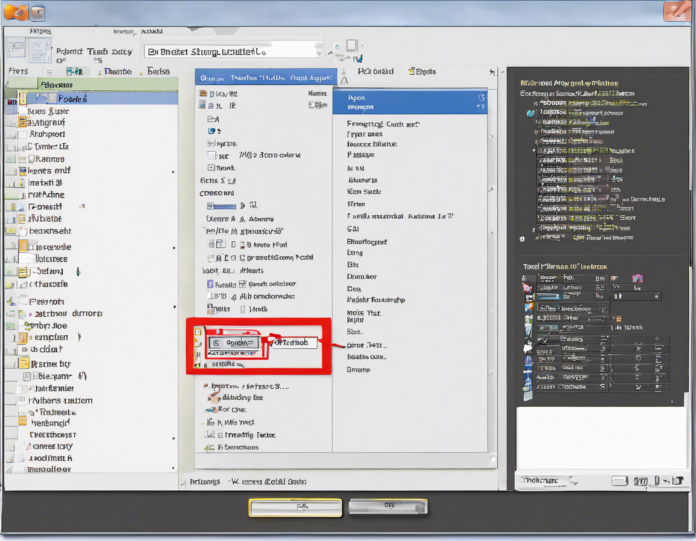
Pivot tables are an incredibly powerful feature in Microsoft Excel that allows users to analyze, summarize, and visualize large amounts of data with ease. However, if you are new to pivot tables, you might be wondering where to find the option to insert a pivot table in Excel. In this article, we will guide you through the process so you can harness the full potential of this tool.
Inserting a Pivot Table in Excel
To insert a pivot table in Excel, you can follow these simple steps:
-
Select Your Data: Before you can create a pivot table, you need to have a dataset ready. Click on any cell within your data range.
-
Go to the Insert Tab: Once you have selected your data, navigate to the “Insert” tab on the Excel ribbon at the top of the screen.
-
Click on PivotTable: In the “Tables” group on the Insert tab, you will see the option for “PivotTable.” Click on this option.
-
Choose Your Data Range: A “Create PivotTable” dialog box will appear. Excel will automatically select the range of your data. Ensure that this range is correct. You can also manually enter the range of data you want to analyze.
-
Select Where to Place the Pivot Table: Choose whether you want the pivot table to be placed in a new worksheet, an existing worksheet, or the same worksheet as your data. Click “OK.”
-
Drag and Drop Fields: Excel will insert a blank pivot table and display the PivotTable Field List pane. You can drag and drop fields from your dataset into the Rows, Columns, Values, and Filters areas of the pivot table to start analyzing your data.
Working with Pivot Tables
Once you have inserted a pivot table in Excel, you can perform various actions to customize and analyze your data:
- Filtering Data: Use the filter buttons in the pivot table to show specific data points.
- Grouping Data: Group dates, numbers, or text fields within the pivot table for better analysis.
- Calculations: Add calculations such as sums, averages, counts, and more to your pivot table.
- Pivot Charts: Create visual representations of your data using pivot charts alongside your pivot table.
Frequently Asked Questions (FAQs)
- Can I create a pivot table from multiple worksheets in Excel?
-
Yes, you can create a pivot table from data located on different worksheets by using the “PivotTable and PivotChart Wizard.”
-
How do I update data in a pivot table?
-
To update data in a pivot table, simply right-click anywhere within the pivot table and select “Refresh.”
-
Can I change the layout and design of a pivot table in Excel?
-
You can customize the layout, design, and formatting of your pivot table using the various options available in the “Design” and “Analyzing” tabs that appear when the pivot table is selected.
-
Are pivot tables dynamic?
-
Yes, pivot tables are dynamic, meaning they will automatically update when the source data changes.
-
Can I use formulas in a pivot table?
- Pivot tables are designed to summarize and analyze data, so you cannot insert formulas directly within the pivot table. However, you can create calculated fields or items to perform calculations.
By following these steps and tips, you can easily find the option to insert a pivot table in Excel and start leveraging this powerful tool to analyze your data more efficiently. Experiment with different features and functionalities to get the most out of your pivot tables and gain valuable insights from your datasets.


